Correlations between plant species and DNA barcode availability

This notebook pulls in data from various sources and makes plots to compare plants species per family to availability of DNA barcodes.

# Set a specific CRAN mirror
options(repos = c(CRAN = "https://cloud.r-project.org/"))

## First check for the required packages, install if needed, and load the libraries.
if (!requireNamespace("BiocManager", quietly = TRUE))
    install.packages("BiocManager")

BiocManager::install("sangerseqR")
remotes::install_github("ropensci/bold")
remotes::install_github("ropensci/taxize")

if (!require("pacman")) install.packages("pacman")
pacman::p_load(maps, ggplot2, dplyr, countrycode, rgbif, data.table, raster, mapproj, sf, glue)

SI Appendix Figure 2A-D: Read in files and summarize for panels A-B.

First we read in the data and make some quick plots.

The combtab data corresponds to the Supplemental Dataset S1 from the publication.

combtab <- read.csv("../data/Kartzinel_et_al_Dataset_S1_20240725.csv")
head(combtab, 2)

   Process.ID        Phylum         Class    Order      Family    Subfamily
1   API120-12 Magnoliophyta Magnoliopsida Lamiales Acanthaceae             
2 CANGI002-17 Magnoliophyta Magnoliopsida Lamiales Acanthaceae Acanthoideae
        Genus                  Species Subspecies Latitude Longitude Country
1 Peristrophe Peristrophe bicalyculata                  NA        NA        
2     Ruellia          Ruellia inflata                  NA        NA  Brazil
  rbcL matK trnL ITS Multiple.markers rbcL.Genbank.accession
1 rbcL                        rbcL---                       
2 rbcL matK      ITS   rbcL-matK--ITS                       
  matK.Genbank.accession trnL.Genbank.accession ITS.Genbank.accession
1                                                                    
2                                                                    

# Round coordiantes to nearest 1 degree
combtab$lat <- as.numeric(as.character(combtab$Latitude))
combtab$lon <- as.numeric(as.character(combtab$Longitude))

# Phylum rank
barplot(sort(table(combtab$Phylum), decreasing=T), main = "Most barcoded Phyla")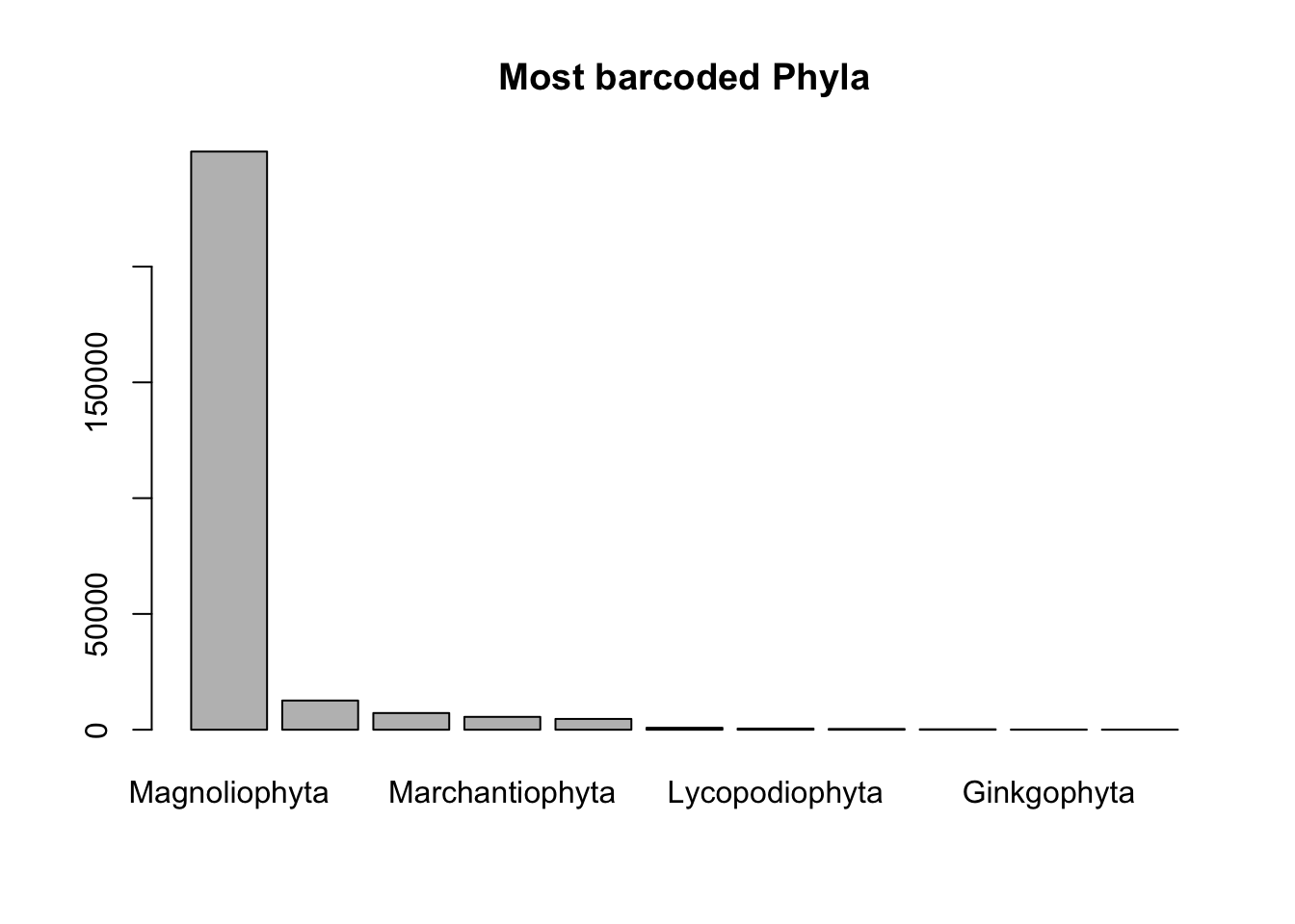

# Family rank
head(sort(table(combtab$Family), decreasing=T), 10)

     Fabaceae       Poaceae   Orchidaceae    Asteraceae      Rosaceae 
        17808         15624         14575         14410          6802 
    Rubiaceae    Cyperaceae     Lamiaceae Euphorbiaceae     Ericaceae 
         6690          6214          5325          4863          4057 

barplot(sort(table(combtab$Family), decreasing=T), main = "Most barcoded Families")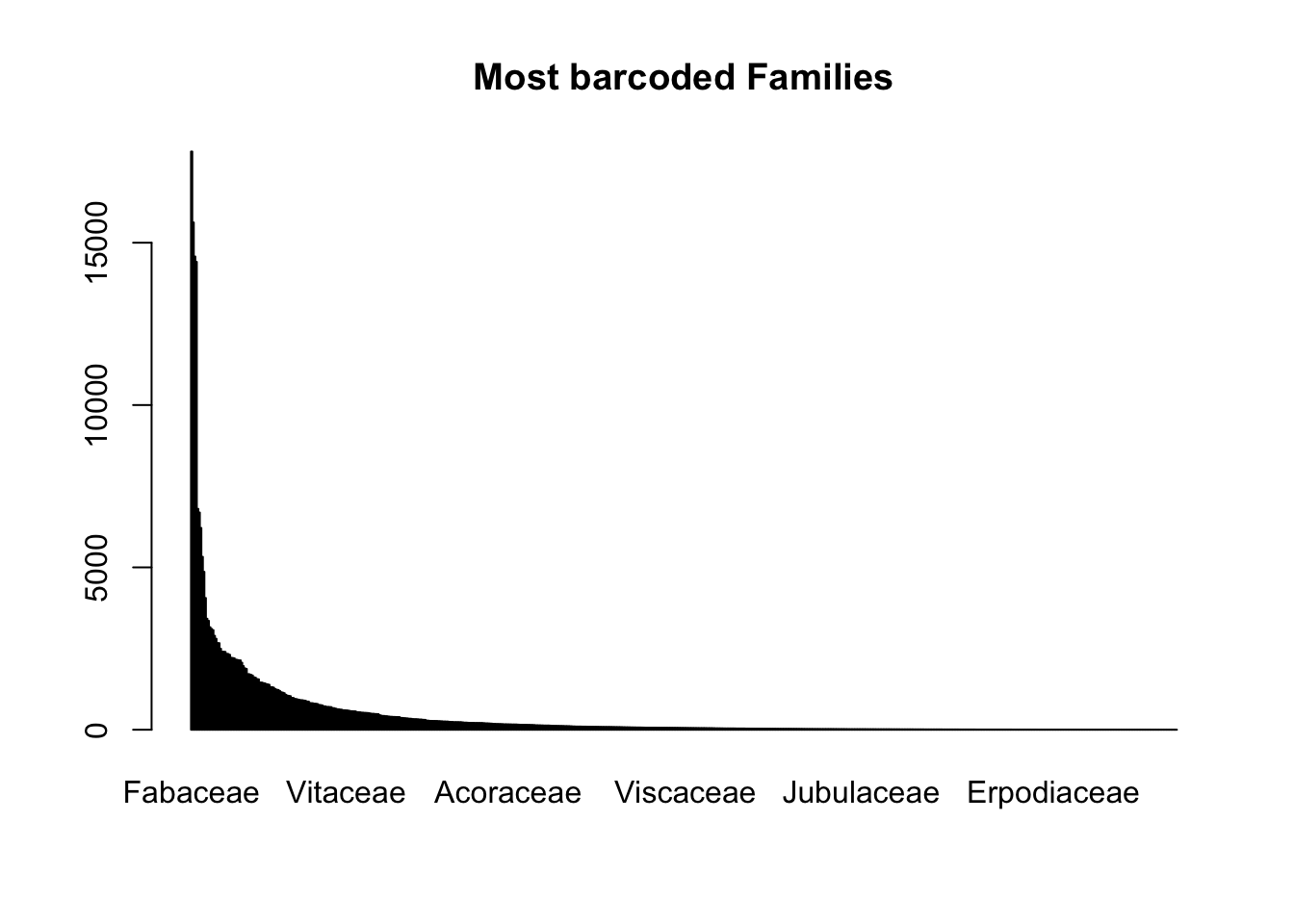

head(table(combtab$Family, combtab$Multiple.markers), 2)

             
              ---ITS --trnL- -matK-- -matK-trnL- #NAME? rbcL--- rbcL---ITS
  Acanthaceae    626       2     130          10      0     192          6
  Achariaceae      2       1      25           0      0     132          0
             
              rbcL--trnL- rbcL--trnL-ITS rbcL-matK-- rbcL-matK--ITS
  Acanthaceae          25              1         285             70
  Achariaceae           0              0         136              6
             
              rbcL-matK-trnL- rbcL-matK-trnL-ITS
  Acanthaceae              77                 16
  Achariaceae               1                  1

# the most barcoded plant species in the world
sort(table(combtab$Species), decreasing=T)[1:5] # by specimens

                                          Bryum argenteum 
                        7495                          551 
         Scorpidium cossonii Acanthorrhynchium papillatum 
                         354                          195 
              Aneura pinguis 
                         195 

Plot family abundances in ITIS and compare with barcodes: this section gives us panels A and B of the figure

The infam data corresponds to the Supplemental Dataset S2 from the publication.

infam <- read.csv("../data/allFamNames.csv")
ITISfamcount <- sort(table(infam$family), decreasing=T)

# Create a useful matrix for summarizing the BOLD counts with respect to ITIS matches
famcountmat <- matrix(0, nrow = length(ITISfamcount), ncol = 9)
colnames(famcountmat)<-c("rank", "ITISfamname", "ITISfamcount", "BOLDspecimencount", "BOLDspeccount", "trnLcount", "rbcLcount", "matKcount", "ITScount")
  famcountmat<-data.frame(famcountmat)
  famcountmat[,1]<-seq(1,length(ITISfamcount))
  famcountmat[,2]<-names(ITISfamcount)
  famcountmat[,3]<-ITISfamcount

# Make count of specimens by family 
combtabfamilycount <- table(combtab$Family)
famcountmat[,4] <- combtabfamilycount[match(famcountmat[,2], names(combtabfamilycount))]

# Make count of species by family
combtabspeciescount <- tapply(combtab$Species, combtab$Family, function(x) length(unique(x)))
famcountmat[,5] <- combtabspeciescount[match(famcountmat[,2], names(combtabspeciescount))]

# Make count of trnL by family
combtabtrnLcount <- tapply(combtab$trnL, combtab$Family, function(x) length(which(x == "trnL")))
famcountmat[,6] <- combtabtrnLcount[match(famcountmat[,2], names(combtabtrnLcount))]
  
# Make count of rbcL by family
combtabrbcLcount <- tapply(combtab$rbcL, combtab$Family, function(x) length(which(x=="rbcL")))
famcountmat[,7] <- combtabrbcLcount[match(famcountmat[,2], names(combtabrbcLcount))]
  
# Make count of matK by family
combtabmatKcount <- tapply(combtab$matK, combtab$Family, function(x) length(which(x=="matK")))
famcountmat[,8] <- combtabmatKcount[match(famcountmat[,2], names(combtabmatKcount))]
  
# Make count of ITS by family
combtabITScount <- tapply(combtab$ITS, combtab$Family, function(x) length(which(x=="ITS")))
famcountmat[,9] <- combtabITScount[match(famcountmat[,2], names(combtabITScount))]

write.csv(famcountmat, "../data/DatasetS2_trnL_rbcL_matK_ITS.csv")

Summarize the data:

get_genera_from_family <- function(family_name) {
  tsn <- get_tsn(family_name, rows = 1, db = "itis")
  
  if (!is.na(tsn)) {
    result <- downstream(tsn, downto = "genus", db = "wfo")
    if (!is.null(result[[1]])) {
      return(result[[1]]$taxonname)
    }
  }
  return(NULL)
}

install.packages("rgbif")

The downloaded binary packages are in
    /var/folders/0y/r_pk_m1j77vbq82t895ph8780000gq/T//RtmpY3Px6a/downloaded_packages

library(rgbif)

# Function to get genera from GBIF
get_genera_gbif <- function(family) {
  res <- name_backbone(name = family, rank = "family")  # Get family details
  if (!is.null(res$usageKey)) {
    # Search for genera within this family
    genera_data <- name_usage(key = res$usageKey, rank = "genus", limit = 100)
    return(unique(genera_data$data$scientificName))
  } else {
    return(NULL)
  }
}

# Example list of plant families
plant_families <- c("Poaceae", "Fabaceae", "Asteraceae", "Orchidaceae", "Rosaceae")

# Retrieve genera for each family
all_genera <- lapply(plant_families, get_genera_gbif)
names(all_genera) <- plant_families

# Print results
print(all_genera)

$Poaceae
[1] "Poaceae"

$Fabaceae
[1] "Fabaceae"

$Asteraceae
[1] "Asteraceae"

$Orchidaceae
[1] "Orchidaceae"

$Rosaceae
[1] "Rosaceae"

# Number of taxa
nrow(famcountmat)

[1] 730

sum(famcountmat$ITISfamcount)

[1] 51925

range(famcountmat$ITISfamcount)

[1]    1 5061

quantile(famcountmat$ITISfamcount)

     0%     25%     50%     75%    100% 
   1.00    1.00    4.00   27.75 5061.00 

median(famcountmat$ITISfamcount)

[1] 4

# Number of family names in ITIS with barcodes
length(which(is.na(famcountmat$BOLDspecimencount) == F))

[1] 609

length(which(is.na(famcountmat$BOLDspecimencount) == F))/nrow(famcountmat)

[1] 0.8342466

# Number of family names ITIS without barcodes
length(which(is.na(famcountmat$BOLDspecimencount)))

[1] 121

length(which(is.na(famcountmat$BOLDspecimencount)))/nrow(famcountmat)

[1] 0.1657534

# Characterize the no-barcode families (i.e., "nbc" families)
nbcfams <- famcountmat[which(is.na(famcountmat$BOLDspecimencount)),]
nbcfams <- nbcfams[order(nbcfams$ITISfamcount),] # reorder by ITIS fam size
head(nbcfams, 2)

    rank      ITISfamname ITISfamcount BOLDspecimencount BOLDspeccount
469  469      Alzateaceae            1                NA            NA
471  471 Ambuchananiaceae            1                NA            NA
    trnLcount rbcLcount matKcount ITScount
469        NA        NA        NA       NA
471        NA        NA        NA       NA

tail(nbcfams, 2)

    rank       ITISfamname ITISfamcount BOLDspecimencount BOLDspeccount
124  124 Balantiopsidaceae           62                NA            NA
45    45   Hydrophyllaceae          203                NA            NA
    trnLcount rbcLcount matKcount ITScount
124        NA        NA        NA       NA
45         NA        NA        NA       NA

sum(nbcfams[,3])

[1] 823

dim(nbcfams)

[1] 121   9

head(sort(nbcfams$ITISfamname), 2) 

[1] "Alzateaceae"      "Ambuchananiaceae"

range(nbcfams$ITISfamcount)

[1]   1 203

hist(nbcfams$ITISfamcount)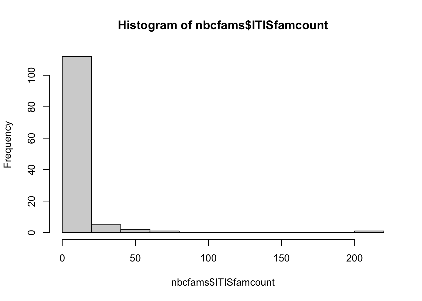

median(nbcfams$ITISfamcount)

[1] 1

head(nbcfams[order(nbcfams[,3]),], 2)

    rank      ITISfamname ITISfamcount BOLDspecimencount BOLDspeccount
469  469      Alzateaceae            1                NA            NA
471  471 Ambuchananiaceae            1                NA            NA
    trnLcount rbcLcount matKcount ITScount
469        NA        NA        NA       NA
471        NA        NA        NA       NA

head(nbcfams[which(nbcfams[,3] == 1),], 2)

    rank      ITISfamname ITISfamcount BOLDspecimencount BOLDspeccount
469  469      Alzateaceae            1                NA            NA
471  471 Ambuchananiaceae            1                NA            NA
    trnLcount rbcLcount matKcount ITScount
469        NA        NA        NA       NA
471        NA        NA        NA       NA

dim(nbcfams[which(nbcfams[,3] == 1),])

[1] 68  9

nrow(nbcfams[which(nbcfams[,3] == 1),])/nrow(nbcfams)

[1] 0.5619835

head(nbcfams[which(nbcfams[,3]<5),], 2)

    rank      ITISfamname ITISfamcount BOLDspecimencount BOLDspeccount
469  469      Alzateaceae            1                NA            NA
471  471 Ambuchananiaceae            1                NA            NA
    trnLcount rbcLcount matKcount ITScount
469        NA        NA        NA       NA
471        NA        NA        NA       NA

dim(nbcfams[which(nbcfams[,3]<5),])

[1] 93  9

nrow(nbcfams[which(nbcfams[,3]<5),])/nrow(nbcfams)

[1] 0.768595

head(nbcfams[which(nbcfams$ITISfamname == "Heliophytaceae"),], 2)

[1] rank              ITISfamname       ITISfamcount      BOLDspecimencount
[5] BOLDspeccount     trnLcount         rbcLcount         matKcount        
[9] ITScount         
<0 rows> (or 0-length row.names)

head(nbcfams[which(nbcfams$ITISfamname == "Calliergonaceae"),], 2)

    rank     ITISfamname ITISfamcount BOLDspecimencount BOLDspeccount trnLcount
203  203 Calliergonaceae           21                NA            NA        NA
    rbcLcount matKcount ITScount
203        NA        NA       NA

# Summarize families in BOLD not in ITIS
boldfamnames <- unique(combtab$Family)
length(boldfamnames) #651

[1] 651

# Families in BOLD not matched by ITIS
nomatchnames <- boldfamnames[which(boldfamnames %in% famcountmat$ITISfamname == F)]
nomatchnames <- nomatchnames[which(nomatchnames != "")]
length(nomatchnames) #42

[1] 42

length(nomatchnames)/length(boldfamnames) #0.06451613

[1] 0.06451613

# Counts of specimens in families in BOLD not matched by ITIS
combtab$family_name <- factor(combtab$Family)
head(sort(table(droplevels(combtab[which(combtab$family_name %in% nomatchnames),]$family_name)), decreasing=T), 2)

Chenopodiaceae  Asphodelaceae 
           818            798 

sum(sort(table(droplevels(combtab[which(combtab$family_name %in% nomatchnames),]$family_name)), decreasing=T))

[1] 3898

sum(sort(table(droplevels(combtab[which(combtab$family_name %in% nomatchnames),]$family_name)), decreasing=T))/nrow(combtab)

[1] 0.01383894

median(sort(table(droplevels(combtab[which(combtab$family_name %in% nomatchnames),]$family_name)), decreasing=T))

[1] 8

# Number of specimens not identified to family
length(which(combtab$family_name == ""))

[1] 0

SI Appendix Figure 2A-D: Plot panels A-B

# Plot family count by specimens: Panel A
plotcorrs <- famcountmat[complete.cases(famcountmat[,3:4]),] 
summary(lm(log(as.numeric(plotcorrs$BOLDspecimencount)) ~ log(as.numeric(plotcorrs$ITISfamcount))))

Call:
lm(formula = log(as.numeric(plotcorrs$BOLDspecimencount)) ~ log(as.numeric(plotcorrs$ITISfamcount)))

Residuals:
    Min      1Q  Median      3Q     Max 
-4.1891 -0.8690  0.1937  0.8946  4.4466 

Coefficients:
                                        Estimate Std. Error t value Pr(>|t|)
(Intercept)                              2.36350    0.07568   31.23   <2e-16
log(as.numeric(plotcorrs$ITISfamcount))  0.82925    0.02606   31.82   <2e-16
                                           
(Intercept)                             ***
log(as.numeric(plotcorrs$ITISfamcount)) ***
---
Signif. codes:  0 '***' 0.001 '**' 0.01 '*' 0.05 '.' 0.1 ' ' 1

Residual standard error: 1.301 on 607 degrees of freedom
Multiple R-squared:  0.6251,    Adjusted R-squared:  0.6245 
F-statistic:  1012 on 1 and 607 DF,  p-value: < 2.2e-16

plotcorrs_ggplot_BOLDspecimen_ITISfamily <- ggplot(
  plotcorrs, aes(x=log(ITISfamcount), y=log(BOLDspecimencount))) + 
  geom_point(pch = 1) + 
  theme_classic() + 
  xlab("Log of ITIS family count") + 
  ylab("Log of BOLD specimen count") + 
  geom_abline(intercept = 0, slope = 1, color = "black", linewidth = 1, linetype = "dashed") + 
  geom_smooth(method = "lm", se=FALSE, linewidth=1, color = "darkgreen") +
  scale_y_continuous(breaks = seq(0,9, by = 3)) + 
  scale_x_continuous(breaks = seq(0,9, by = 3))
plotcorrs_ggplot_BOLDspecimen_ITISfamily

`geom_smooth()` using formula = 'y ~ x'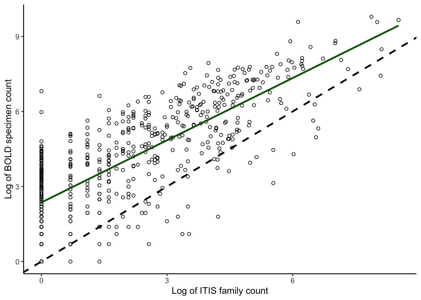

#ggsave("plotcorrs_ggplot_BOLDspecimen_ITISfamily.pdf", plotcorrs_ggplot_BOLDspecimen_ITISfamily, width = 10, height = 8, units = "cm")
        
# Summary stats for panel A
plotcorrs_summary <- plotcorrs %>% dplyr::summarize(sumspecimens = sum(BOLDspecimencount))
plotcorrs_summary

  sumspecimens
1       277771

# Plot family count by species: PANEL B
plotcorrs_ggplot_BOLDspecies_ITISfamily <- ggplot(
  plotcorrs, aes(x=log(ITISfamcount), y=log(BOLDspeccount))) + 
  geom_point(pch = 1) + 
  theme_classic() + 
  xlab("Log of ITIS family count") + 
  ylab("Log of BOLD species count") + 
  geom_abline(intercept = 0, slope = 1, color = "black", linewidth = 1, linetype = "dashed") + 
  geom_smooth(method = "lm", se=FALSE, linewidth=1, color = "darkgreen") +
  scale_y_continuous(breaks = seq(0,9, by = 3)) + scale_x_continuous(breaks = seq(0,9, by = 3))
plotcorrs_ggplot_BOLDspecies_ITISfamily 

`geom_smooth()` using formula = 'y ~ x'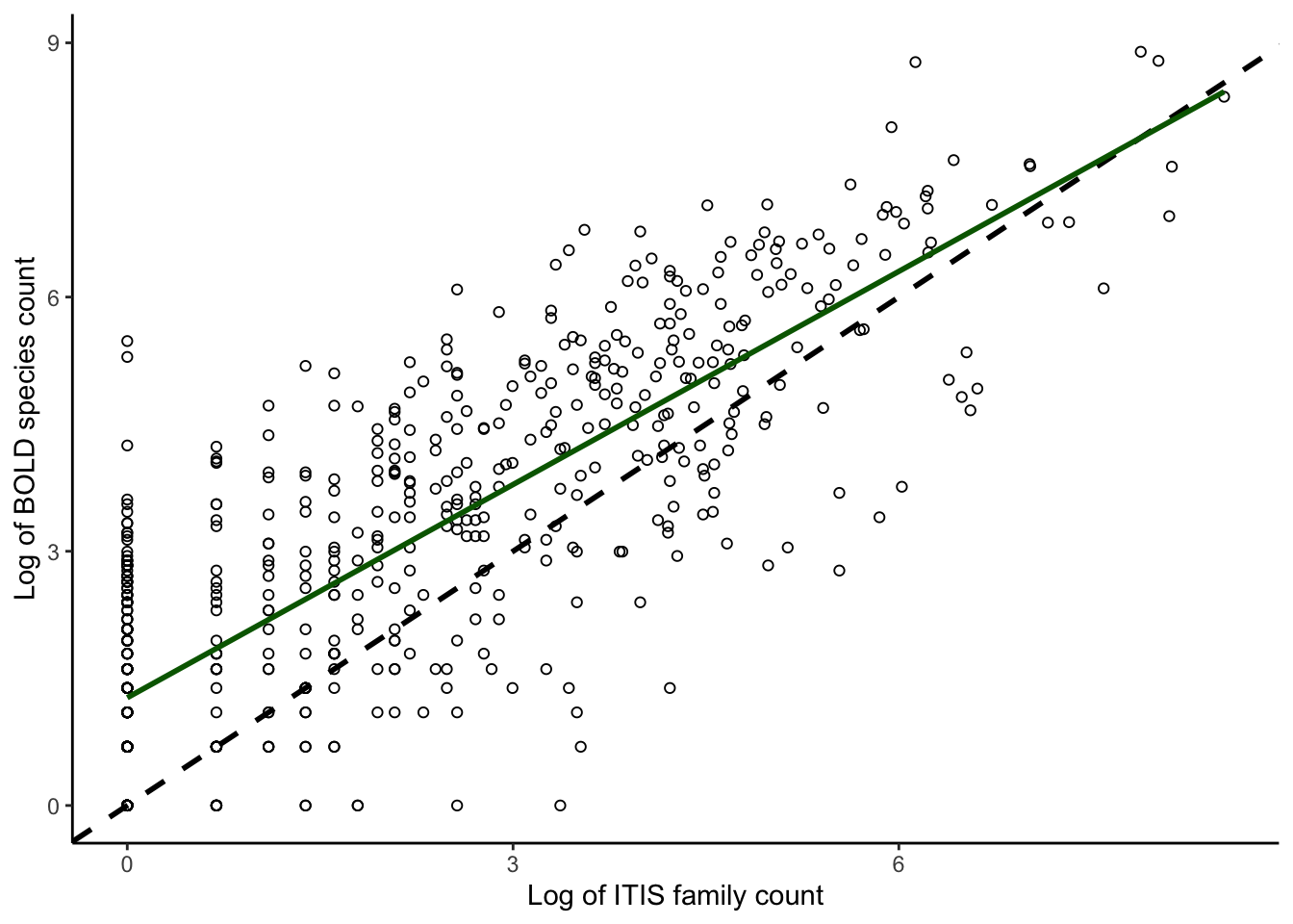

#ggsave("plotcorrs_ggplot_BOLDspecies_ITISfamily.pdf", plotcorrs_ggplot_BOLDspecies_ITISfamily, width = 10, height = 8, units = "cm")
        
#summary stats for panel B
plotcorrs_summary <- plotcorrs %>% summarize(sumspecies = sum(BOLDspeccount))
plotcorrs_summary

  sumspecies
1     101674

SI Appendix Figure 2A-D: Read in files and summarize for panels C-D.

Now read in the data from downloading all trnL P6 data from the European Nucleotide Archive at EMBL-EBI. More details for the download can be found in the “Building the datasets” section of the Methods in the publication. This data corresponds to dataset S3 in the Supplement.

emblp6 <- read.csv("../data/Kartzinel_et_al_Dataset_S3_20240725.csv")
nrow(emblp6)

[1] 157020

length(unique(emblp6$trnL.P6.sequence)) # number of unique sequences 

[1] 21467

#levels(factor(emblp6$Family)) # uncomment and run to print out all the family names
length(unique(emblp6$Family))

[1] 666

157020/5324 # fold difference between number in BOLD vs EMBL

[1] 29.49286

emblp6_nofamily <- subset(emblp6, Family == "")

# Build the same kind of matrix as above
famcountmatp6 <- matrix(0, nrow = length(ITISfamcount), ncol = 5)
colnames(famcountmatp6) <- c("rank", "ITISfamname", "ITISfamcount", "p6seqcount", "p6speccount")
famcountmatp6 <- data.frame(famcountmatp6)
famcountmatp6[,1] <- seq(1,length(ITISfamcount))
famcountmatp6[,2] <- names(ITISfamcount)
famcountmatp6[,3] <- ITISfamcount
length(unique(emblp6$Family))

[1] 666

#unique(emblp6$family_name) # uncomment to print out all the family names

write.csv(famcountmatp6, "../data/DatasetS2_P6_additions.csv")

# Make count of specimens by family
emblp6count <- table(emblp6$Family)
famcountmatp6[,4] <- emblp6count[match(famcountmatp6[,2], names(emblp6count))]
length(emblp6count)

[1] 666

sum(emblp6count)

[1] 157020

# Make count of species by family
emblp6speciescount <- tapply(emblp6$Species, emblp6$Family, function(x) length(unique(x)))
famcountmatp6[,5] <- emblp6speciescount[match(famcountmatp6[,2], names(emblp6speciescount))]

Summarize the data:

# Number of taxa
nrow(famcountmatp6)

[1] 730

sum(famcountmatp6$ITISfamcount)

[1] 51925

range(famcountmatp6$ITISfamcount)

[1]    1 5061

quantile(famcountmatp6$ITISfamcount)

     0%     25%     50%     75%    100% 
   1.00    1.00    4.00   27.75 5061.00 

median(famcountmatp6$ITISfamcount)

[1] 4

# Number of family names in ITIS with barcodes
length(which(is.na(famcountmatp6$p6seqcount) == F))

[1] 611

length(which(is.na(famcountmatp6$p6seqcount) == F))/nrow(famcountmatp6)

[1] 0.8369863

# Number of family names ITIS without barcodes
length(which(is.na(famcountmatp6$p6seqcount)))

[1] 119

length(which(is.na(famcountmatp6$p6seqcount)))/nrow(famcountmatp6)

[1] 0.1630137

# Characterize the no-barcode families
nbcfamsp6 <- famcountmatp6[which(is.na(famcountmatp6$p6seqcount)),]
nbcfamsp6 <- nbcfamsp6[order(nbcfamsp6$ITISfamcount),] # reorder by ITIS fam size
head(nbcfamsp6, 2)

    rank   ITISfamname ITISfamcount p6seqcount p6speccount
469  469   Alzateaceae            1         NA          NA
472  472 Anarthriaceae            1         NA          NA

tail(nbcfamsp6, 2)

    rank      ITISfamname ITISfamcount p6seqcount p6speccount
129  129  Selaginellaceae           56         NA          NA
15    15 Xanthorrhoeaceae          658         NA          NA

sum(nbcfamsp6[,3])

[1] 1069

dim(nbcfamsp6)

[1] 119   5

head(sort(nbcfamsp6 $ITISfamname), 2)

[1] "Alzateaceae"  "Amphidiaceae"

range(nbcfamsp6 $ITISfamcount)

[1]   1 658

hist(nbcfamsp6 $ITISfamcount)

median(nbcfamsp6 $ITISfamcount)

[1] 1

head(nbcfamsp6[order(nbcfamsp6[,3]),], 2)

    rank   ITISfamname ITISfamcount p6seqcount p6speccount
469  469   Alzateaceae            1         NA          NA
472  472 Anarthriaceae            1         NA          NA

head(nbcfamsp6[which(nbcfamsp6[,3]==1),], 2)

    rank   ITISfamname ITISfamcount p6seqcount p6speccount
469  469   Alzateaceae            1         NA          NA
472  472 Anarthriaceae            1         NA          NA

dim(nbcfamsp6[which(nbcfamsp6[,3]==1),])

[1] 76  5

nrow(nbcfamsp6[which(nbcfamsp6[,3]==1),])/nrow(nbcfamsp6)

[1] 0.6386555

head(nbcfamsp6[which(nbcfamsp6[,3]<5),], 2)

    rank   ITISfamname ITISfamcount p6seqcount p6speccount
469  469   Alzateaceae            1         NA          NA
472  472 Anarthriaceae            1         NA          NA

dim(nbcfamsp6[which(nbcfamsp6[,3]<5),])

[1] 100   5

nrow(nbcfamsp6[which(nbcfamsp6[,3]<5),])/nrow(nbcfamsp6)

[1] 0.8403361

head(nbcfamsp6[which(nbcfamsp6 $ITISfamname=="Heliophytaceae"),], 2)

[1] rank         ITISfamname  ITISfamcount p6seqcount   p6speccount 
<0 rows> (or 0-length row.names)

head(nbcfamsp6[which(nbcfamsp6 $ITISfamname=="Calliergonaceae"),], 2)

[1] rank         ITISfamname  ITISfamcount p6seqcount   p6speccount 
<0 rows> (or 0-length row.names)

# Summarize families in embl not in ITIS
p6famnames <- unique(emblp6$Family)
length(p6famnames)

[1] 666

# Families in embl not matched by ITIS
nomatchnamesp6 <- p6famnames[which(p6famnames %in% famcountmatp6$ITISfamname == F)]
nomatchnamesp6 <- nomatchnamesp6[which(nomatchnamesp6 != "")]
length(nomatchnamesp6)

[1] 55

length(nomatchnamesp6)/length(p6famnames)

[1] 0.08258258

# Counts of specimens in families in embl not matched by ITIS
emblp6$family_name <- factor(emblp6$Family)
head(sort(table(droplevels(emblp6[which(emblp6 $family_name %in% nomatchnamesp6),]$family_name)), decreasing=T), 2)

 Hyacinthaceae Chenopodiaceae 
           672            347 

sum(sort(table(droplevels(emblp6[which(emblp6 $family_name %in% nomatchnamesp6),]$family_name)), decreasing=T))

[1] 1809

sum(sort(table(droplevels(emblp6[which(emblp6 $family_name %in% nomatchnamesp6),]$family_name)), decreasing=T))/nrow(combtab)

[1] 0.006422432

median(sort(table(droplevels(combtab[which(combtab$family_name %in% nomatchnamesp6),]$family_name)), decreasing=T))

[1] 8

# Number of specimens not identified to family
length(which(emblp6$family_name == ""))

[1] 0

Write out the Supplemental Dataset S2

ds_s2 <- merge(famcountmat, famcountmatp6, by=c("rank","ITISfamname","ITISfamcount"))
write.csv(ds_s2, glue("../data/Kartzinel_et_al_Dataset_S2_{params$today}.csv"))

SI Appendix Figure 2A-D: Plot panels C-D

# Plot correlations - family count by specimens: Panel C
plotcorrs <- famcountmatp6[complete.cases(famcountmatp6[,3:4]),]
plotcorrs_ggplot_family_sequences <- ggplot(
  plotcorrs, aes(x=log(ITISfamcount), y=log(p6seqcount))) + 
  geom_point(pch = 1) + 
  theme_classic() + 
  xlab("Log of ITIS family count") + 
  ylab("Log of trnL-P6 sequence count") + 
  geom_abline(intercept = 0, slope = 1, color = "black", linewidth = 1, linetype = "dashed") + 
  geom_smooth(method = "lm", se=FALSE, linewidth=1, color = "darkgreen") +
  scale_y_continuous(breaks = seq(0,9, by = 3)) + 
  scale_x_continuous(breaks = seq(0,9, by = 3))
plotcorrs_ggplot_family_sequences

`geom_smooth()` using formula = 'y ~ x'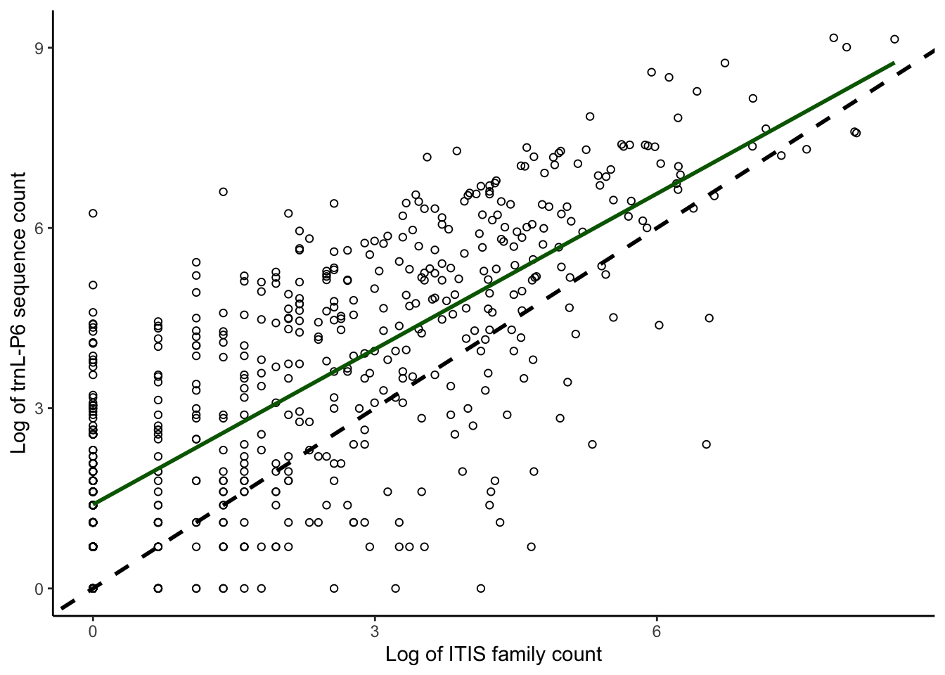

#ggsave("plotcorrs_ggplot_family_sequences.pdf", plotcorrs_ggplot_family_sequences, width = 10, height = 8, units = "cm")

# Summarize for panel C
plotcorrs_summary <- plotcorrs %>% dplyr::summarize(sumP6sequences = sum(p6seqcount))
plotcorrs_summary

  sumP6sequences
1         155211

# Family count by species: Panel D
plotcorrs_ggplot_family_sequencespecies <- ggplot(
  plotcorrs, aes(x=log(ITISfamcount), y=log(p6speccount))) + 
  geom_point(pch = 1) + 
  theme_classic() + 
  xlab("Log of ITIS family count") + 
  ylab("Log of trnL-P6 species count") + 
  geom_abline(intercept = 0, slope = 1, color = "black", linewidth = 1, linetype = "dashed") + 
  geom_smooth(method = "lm", se=FALSE, linewidth=1, color = "darkgreen")  +
  scale_y_continuous(breaks = seq(0,9, by = 3)) + 
  scale_x_continuous(breaks = seq(0,9, by = 3))
plotcorrs_ggplot_family_sequencespecies         

`geom_smooth()` using formula = 'y ~ x'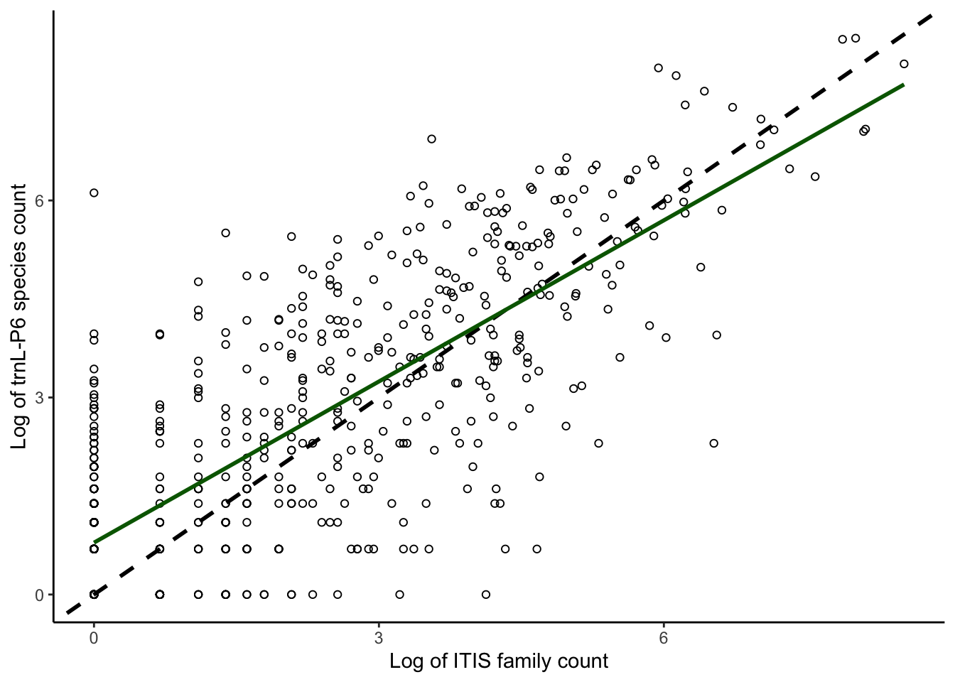

#ggsave("plotcorrs_ggplot_family_sequencespecies.pdf", plotcorrs_ggplot_family_sequencespecies, width = 10, height = 8, units = "cm")

# Summarize for panel D
plotcorrs_summary <- plotcorrs %>% summarize(sump6speccount = sum(p6speccount))
plotcorrs_summary

  sump6speccount
1          69873