## First check for the required packages, install if needed, and load the libraries.
if (!requireNamespace("BiocManager", quietly = TRUE))
    install.packages("BiocManager")

BiocManager::install("sangerseqR")
remotes::install_github("ropensci/bold")
remotes::install_github("ropensci/taxize")

if (!require("pacman")) install.packages("pacman")
pacman::p_load(maps, ggplot2, dplyr, countrycode, rgbif, data.table, raster, mapproj, sf)Coverage by country
This notebook analyzes the counts of barcodes by country and plots the results.
SI Figure S1: Map of country counts
Start with some data cleaning.
combtab <- read.csv("../data/BoldPhyla_to_Families_combtab_v4.csv")
head(combtab, 2)
X.1 X processid institution_storing phylum_taxID
1 1 1 API120-12 Sri Ramaswamy Memorial University 12
2 2 2 CANGI002-17 Museu Paraense Emilio Goeldi 12
phylum_name class_taxID class_name order_taxID order_name family_taxID
1 Magnoliophyta 41 Magnoliopsida 121216 Lamiales 148533
2 Magnoliophyta 41 Magnoliopsida 121216 Lamiales 148533
family_name subfamily_taxID subfamily_name genus_taxID genus_name
1 Acanthaceae NA 415894 Peristrophe
2 Acanthaceae 264310 Acanthoideae 148534 Ruellia
species_taxID species_name subspecies_taxID subspecies_name
1 494465 Peristrophe bicalyculata NA
2 632816 Ruellia inflata NA
collectiondate_start collectiondate_end lat lon coord_source coord_accuracy
1 NA NA NA NA NA
2 NA NA NA NA NA
elev country province_state region sector exactsite rbcL matK trnL ITS2
1 NA rbcL
2 NA Brazil Para rbcL matK ITS
multi gb_rbcL gb_matK gb_trnL gb_ITS
1 rbcL---
2 rbcL-matK--ITS # Round coordiantes to nearest 1 degree
combtab$lat <- as.numeric(as.character(combtab$lat))
combtab$lon <- as.numeric(as.character(combtab$lon))
# ggplot wrapper of map()
world_map <- map_data("world")
# Build a dataframe / matrix of country counts to plot
myCodes <- data.frame(table(combtab$country))
colnames(myCodes)<-c("country", "n")
# Convert country names to "Getty Thesaurus" names for BOLD
myCodes$country <- countrycode(myCodes$country, "country.name", "country.name")
myCodes$country[which(myCodes$country=="United States")]<-"USA"
myCodes$country[which(myCodes$country=="United Kingdom")]<-"UK"
myCodes$country[which(myCodes$country=="Congo - Kinshasa")]<-"Democratic Republic of the Congo"
myCodes$country[which(myCodes$country=="Congo - Brazzaville")]<-"Republic of Congo"
myCodes$country[which(myCodes$country=="British Virgin Islands")]<-"Virgin Islands"
myCodes$country[which(myCodes$country=="Bosnia & Herzegovina")]<-"Bosnia and Herzegovina"
myCodes$country[which(myCodes$country=="São Tomé & Príncipe")]<-"Sao Tome and Principe"
myCodes$country[which(myCodes$country=="Trinidad & Tobago")]<-"Trinidad" #Tobago is a separate entity in maps
myCodes$country[which(myCodes$country=="North Macedonia")]<-"Macedonia"
myCodes$country[which(myCodes$country=="Myanmar (Burma)")]<-"Myanmar"
myCodes$country[which(myCodes$country=="Côte d’Ivoire")]<-"Ivory Coast"
myCodes$country[which(myCodes$country=="Czechia")]<-"Czech Republic"
myCodes$country[which(myCodes$country=="Réunion")]<-"Reunion"
myCodes$country[which(myCodes$country=="St. Helena")]<-"Saint Helena"
myCodes$country[which(myCodes$country=="Eswatini")]<-"Swaziland" Map country-level barcode intensity.
# Map for country-level intensity
myCodes <- myCodes[is.na(myCodes$country)==F,]

ggpoliticalboundaries <- ggplot(myCodes) +
  geom_map(dat = world_map, map = world_map, aes(map_id = region), fill = "white", color = "#7f7f7f", linewidth = 0.25)  +
  geom_map(map = world_map, aes(map_id = country, fill = n), linewidth = 0.25) +
  scale_fill_gradient(low = "#fff7bc", high = "#cc4c02", name = "Worldwide specimens") + scale_x_continuous(breaks = seq(-180, 180, by = 60)) +
  scale_y_continuous(breaks = seq(-90, 90, by = 45)) +
  expand_limits(x = world_map$long, y = world_map$lat) +
  theme_classic() +
  ylab("") +
  xlab("") +
  theme(legend.position = "none") +
  geom_hline(yintercept = 0, color = "black", linewidth = 0.5) +
  geom_hline(yintercept = 23.5, color = "black", linetype = "dashed") +
  geom_hline(yintercept = -23.5, color = "black", linetype = "dashed")
ggpoliticalboundaries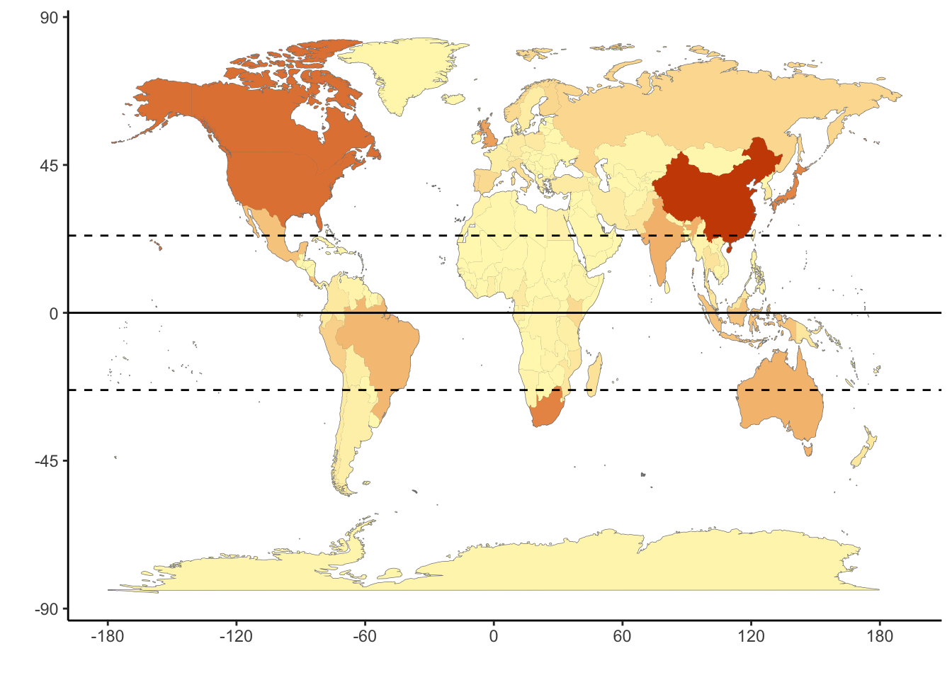
#ggsave("ggpoliticalboundaries_20240626_1.pdf", ggpoliticalboundaries, width = 13, height = 8.6, units = "cm")Distribution of country bias - lineplot.
# Line plot with country counts
countrycounts_line <- ggplot(myCodes, aes(x = reorder(country, -n), y = n, group = 1)) +
  geom_line() +
  theme_classic() +
  xlab("") +
  ylab("") +
  theme(axis.title.x=element_blank(), axis.text.x=element_blank(), axis.ticks.x=element_blank())
countrycounts_line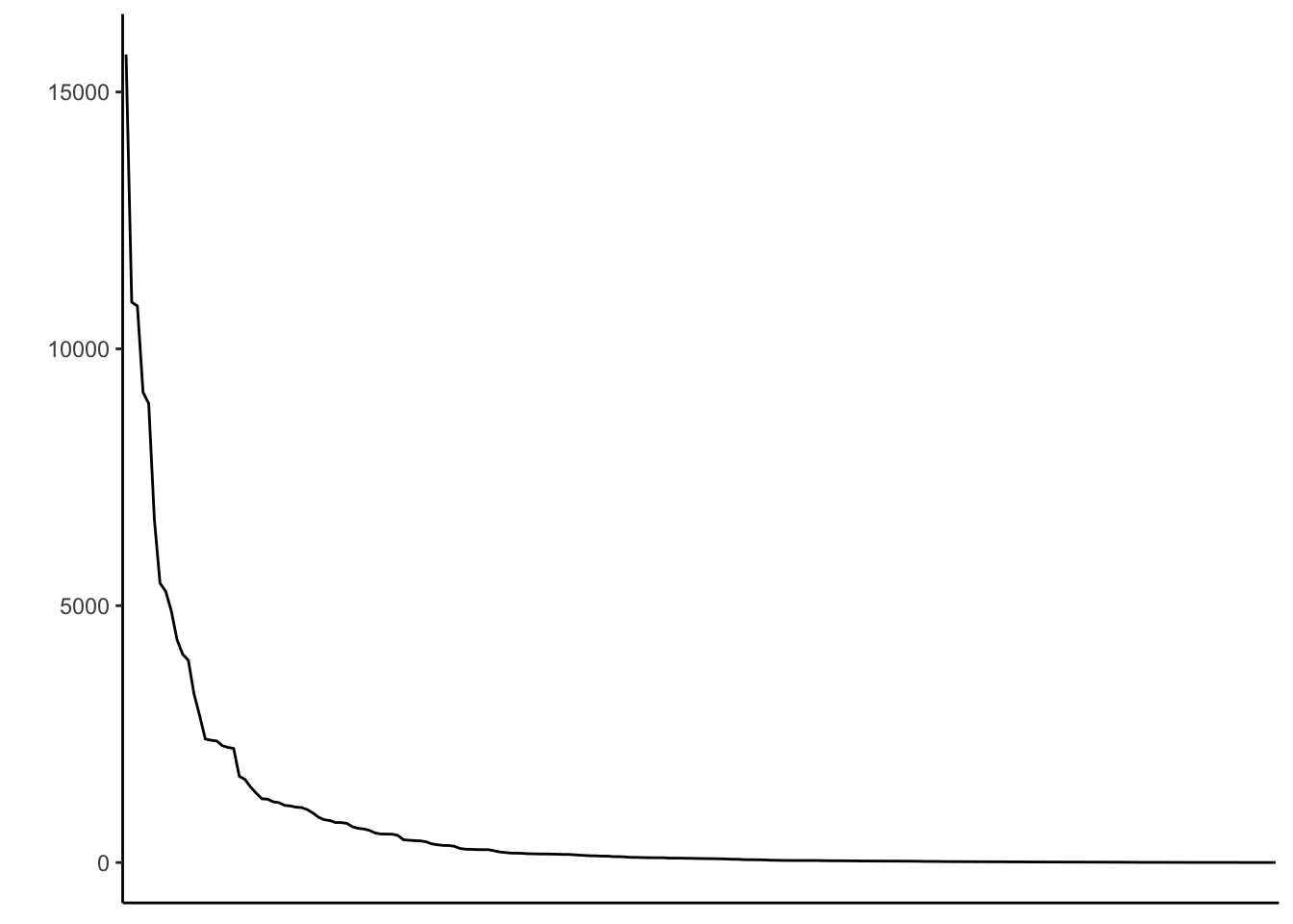
#ggsave("countrycounts_20240626.pdf", countrycounts, width = 8, height = 4, units = "cm")Print dataframe with countries having less than 10 barcodes.
# Summarize number of countries with <10
myCodes_less_than_10 <- subset(myCodes, n <10) %>%
  arrange(desc(n))
myCodes_less_than_10
country n
1 Cape Verde 9
2 Eritrea 9
3 Sierra Leone 9
4 Trinidad 9
5 Guam 8
6 Mayotte 8
7 South Georgia & South Sandwich Islands 8
8 Virgin Islands 7
9 Falkland Islands 7
10 North Korea 7
11 Cook Islands 6
12 United Arab Emirates 6
13 Kosovo 5
14 Belarus 4
15 Chad 4
16 Guinea-Bissau 4
17 Kuwait 4
18 Palau 4
19 Bermuda 3
20 Faroe Islands 3
21 Saint Helena 3
22 Tonga 3
23 Djibouti 2
24 Gambia 2
25 Grenada 2
26 Lithuania 2
27 Maldives 2
28 Niger 2
29 Northern Mariana Islands 2
30 St. Lucia 2
31 San Marino 2
32 Antigua & Barbuda 1
33 Aruba 1
34 Mauritania 1
35 Moldova 1
36 Niue 1
37 St. Vincent & Grenadines 1
38 South Sudan 1